A colleague recently asked me how to fit a spline with a point constraint in a Cox proportional hazards (PH) model. After realizing that his response was interval censored I found that mgcv::cox.ph couldn't be used, as the right censoring is specified as a 0-weight in the syntax (event as 1). I quickly looked into other ways to estimate a penalized spline from the mgcv framework, and since a penalized spline can be rewritten as a random effect I needed to find another package that could estimate mixed Cox PH models, with a Surv object describing the response (which allows for interval censoring). One package fulfilling those criteria is coxme, which also support a ridge regression shrinkage for variables, which we will see is especially well suited for estimating penalized splines in a random effect setting.

First, we load some package:

pacman::p_load(tidyverse,
               survival, 
               coxme, 
               mgcv,
               patchwork)

We will work with the time until death futime (or last contact in case of censoring) in the mgus2 dataset in survival, and use creat as a non-linear predictor.

survival::mgus2 %>% drop_na(creat) -> work_dataset

We construct a smooth object, which we will convert into a random effect, such that the spline $f(x)$ can be written as $\mathbf{f}=\mathbf{X}^{\prime} \boldsymbol{\beta}^{\prime}+\mathbf{Z} \mathbf{b}$, where $\mathbf{b} \sim N\left(\mathbf{0}, \mathbf{I} \sigma_{b}^{2}\right)$. This means that we will have one part of the spline that is regarded as a "fixed effect" in the model, and one part as a set of "random effects" which also shares their variance and are uncorrelated. This happens to be the same thing as a ridge regression, and in coxme the latter can be done via the shrinkage syntax, (variables|1) which impose a ridge shrinkage structure on the variables, which is equivalent to $\mathbf{b} \sim N\left(\mathbf{0}, \mathbf{I} \sigma_{b}^{2}\right)$.

This is called the natural parameterization of a spline, and in this case (I think it is due to the identity matrix as a penalty), it is the same as the original parameterization. The only difference is that in this natural parameterization, the $b$s are in a different order, which will be reordered to the original order in the last row in the following code block. The "fixed effect" part is called the null space, and the "random effect" part is called the penalized space.

sm <- smoothCon(
  s(creat, k = 30, pc = 12.5),
  # dimension of basis: 30, point constraint 12.5
  data = work_dataset,
  absorb.cons = TRUE,
  # identifiability constraints absorbed into the basis
  diagonal.penalty = TRUE
  # the spline is reparameterized to turn the penalty into an identity matrix
)[[1]]

smooth2random(sm, "", type = 2) -> re

re$Xf -> null_space

re$rand$Xr %*% re$trans.U[-ncol(re$trans.U), -ncol(re$trans.U)] ->
  penalized_space # Reorder the matrix of the random effect part

After that we will first fit the model with mgcv, and then with coxme, and afterwards compare the estimates. The spline will be a 30 dimensional basis rank-reduced think plate spline, with a point constraint at $12.5$, i.e. the spline will evaluate to zero in that point. This is useful so that we have a fixed reference point for the hazard ratio. We also prepare a plot of the estimated spline from mgcv.

gam(data = work_dataset,
    formula = futime ~ s(creat, k = 30, pc = 12.5),
    weights = death,
    method = "REML",
    family = cox.ph) -> 
  gam_model

gam_model %>%
  gratia::draw(fun = exp) %>%
  .$data %>%
  ggplot(aes(x = creat,
             y = est,
             ymin = lower,
             ymax = upper)) +
  geom_line() +
  geom_ribbon(alpha = .3) +
  scale_y_continuous(limits = c(0, 8)) +
  labs(title = "mgcv", 
       y = "Hazard ratio") -> 
  plot1

coxme(formula = Surv(time = futime, event = death) ~ null_space + (penalized_space | 1), 
      data = work_dataset) -> 
  test_model

To plot the estimated spline from coxme we need to extract the estimated coefficients for the spline, and its covariance matrix. We setup a "prediction matrix" that tells us how the bases are evaluated at each value for creat, where we take the values from the grid from gratia::draw. As the estimated coefficients are in the same order as the bases in the prediction matrix, we matrix multiply them to get the prediction, since $\hat{f} (x)=\sum_{k=1}^{M} \hat{\beta_{k}} g_{k}(x)$, where $g_{k}$ is each individual basis function. We also extract the covariance matrix for the coefficients.

Xp <- PredictMat(sm, plot1$data)

c(test_model$frail$`1`, coef(test_model)["null_space"]) -> beta_hat

Xp%*%as.vector(beta_hat) -> pred_spline

V <- test_model$variance 
# works if there are no fixed effects as they are in same order as in Xp

The standard error of a fixed point of an estimated spline is $\operatorname{diag}\left(X_{p} \hat{V} X_{p}^{\prime}\right)^{1 / 2}$ or equivalently (and more efficient) in R: $\operatorname{row} \operatorname{Sums}\left(X_{p} \cdot\left(X_{p} \hat{V}\right)\right)^{1 / 2}$ . This is enough to create a plot for the spline estimated with coxme.

plot1$data %>% 
  mutate(y = pred_spline, 
         y_se = sqrt(rowSums(Xp * (Xp %*% V)))) %>% #Xp is also based on plot1$data
  mutate(y_min = y-1.96*y_se, 
         y_max = y+1.96*y_se,
         across(c(y,y_min, y_max), exp)) %>% 
  ggplot(aes(x = creat, 
             y = y, 
             ymin = y_min, 
             ymax = y_max))+
  geom_line()+
  geom_ribbon(alpha=.3)+
  scale_y_continuous(limits = c(0, 8))+
  labs(title = "coxme", y = NULL) -> plot2

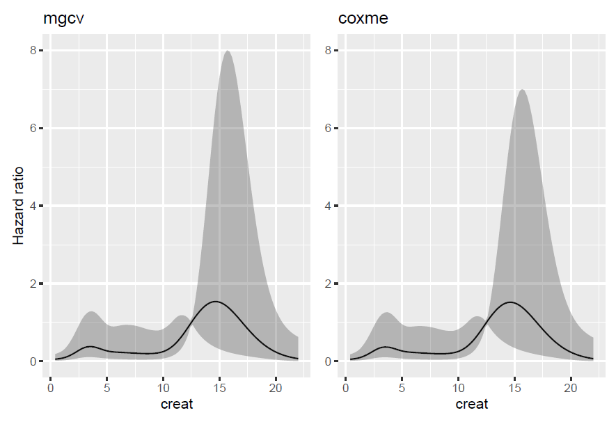
We compare the two estimated splines and see that they are roughly equal. The coxme fit seems to have a bit lower standard errors. This might be due to a biased estimation of the variance for the "shrinkage" in coxme as it seems to be estimated with maximum likelihood rather than restricted maximum likelihood. It might just also be a non-significant (in a practical sense) difference. I actually don't know, but as it seems to mainly affect parts of the function where the uncertainty is high, it is probably a minor concern. Small numeric differences also gets scaled up due to the exponentiation of the estimated spline to get the hazard ratio on the y-axis.

These confidence bands also have a somewhat peculiar interpretation, as its frequentist properties are for the whole function, and not the specific points it is evaluated at. For simultaneous confidence bands, it is together with my former blog post on simultaneous confidence intervals left as an exercise to the reader.

It should also be noted that this code only works out of the box with the rank-reduced thin plate spline (which is the default in mgcv). Smaller adjustments have to be made if fixed/random effects and/or splines are added to the model.

(plot1+plot2)